Table of content :

• Deathcross
• Trend following RSI
• Advanced rend following RSI

Backtesting - Deathcross

Données

df = pd.read_csv('btceur-2h.csv')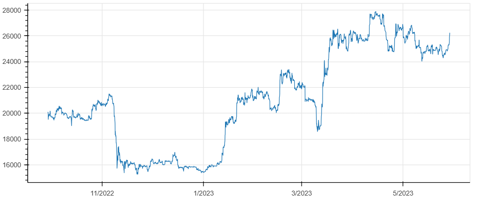

Moyennes mobiles

fast = ta.EMA(df['close'], timeperiod = 20)
slow = ta.SMA(df['close'], timeperiod = 200)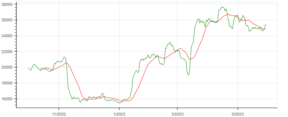

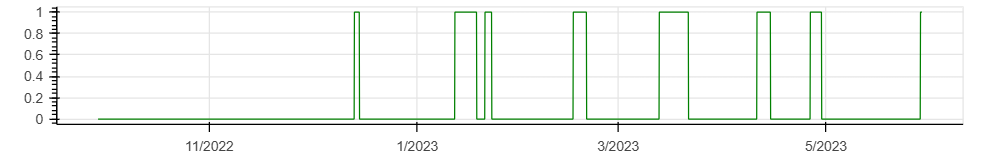
Positions

position = fast > slow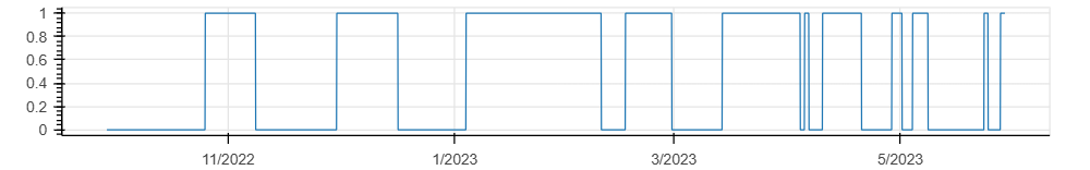

Rendement en HODL

returns_hodl = np.log(df.close / df.close.shift())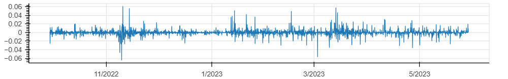

Rendement stratégie

returns_strat = returns_hodl * (position.shift() == 1)
returns_fee = np.log(1 - 0.0025) * (position != position.shift())
returns_netto = returns_strat + returns_fee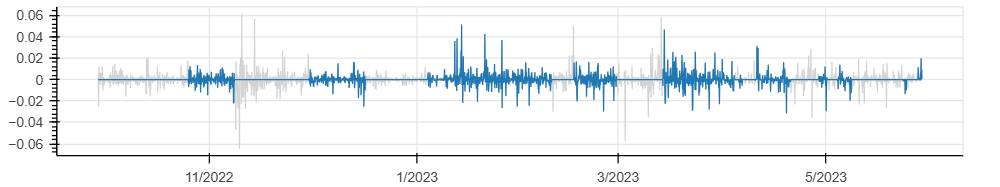

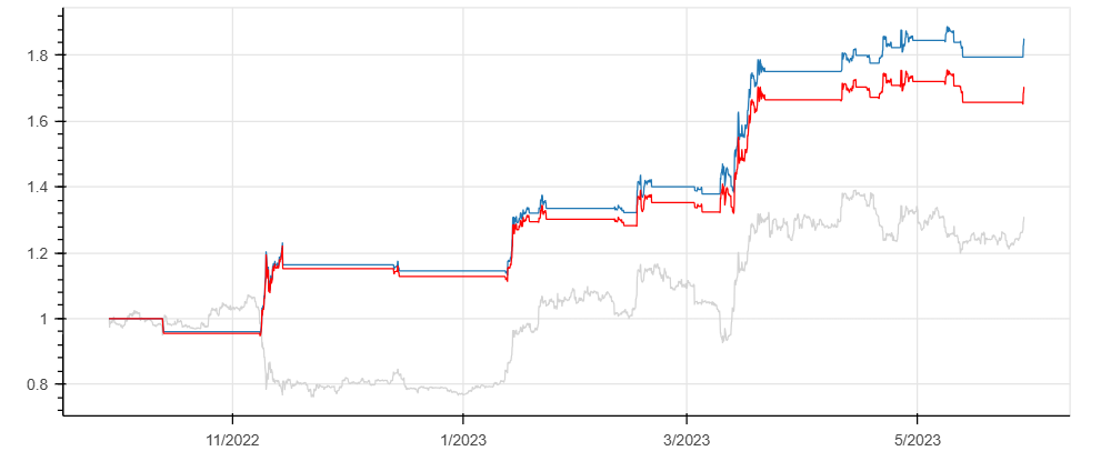
Rendement net cumulé

returns_netto_cumul = np.exp(returns_netto.cumsum())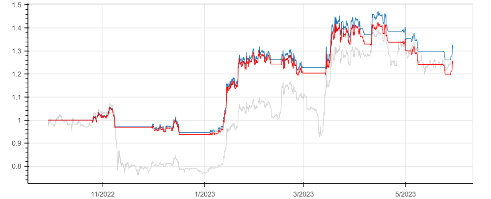

Code

# coding: utf-8

import numpy as np
import pandas as pd
import talib as ta

df = pd.read_csv('btceur-2h.csv')

# strategy
fast = ta.EMA(df['close'], timeperiod = 20)
slow = ta.SMA(df['close'], timeperiod = 200)

position = fast > slow

# returns
returns_hodl = np.log(df.close / df.close.shift())
returns_strat = returns_hodl * (position.shift() == 1)
returns_fee = np.log(1 - 0.0025) * (position != position.shift())
returns_netto = returns_strat + returns_fee
print('Returns: ', np.exp(returns_netto.sum()))

# graphs
from bokeh.plotting import figure,show
from bokeh.layouts import column,row

df['date'] = pd.to_datetime(df.time, unit='s')

fig0 = figure(height=325, width=800, x_axis_type='datetime')
fig0.line(df.date, df.close)

fig1 = figure(height=325, width=800, x_axis_type='datetime')
#fig1.line(df.date, df.close)
fig1.line(df.date, slow, color='red')
fig1.line(df.date, fast, color='green')

fig2 = figure(height=125, width=800, x_axis_type='datetime')
fig2.line(df.date, position)

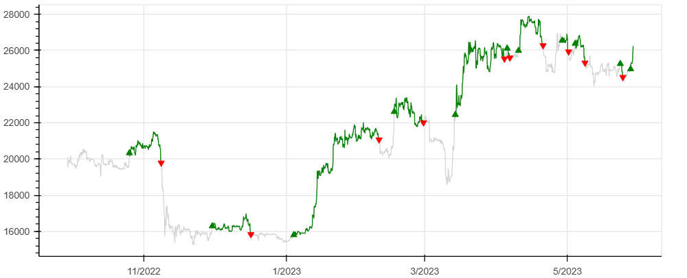
fig3 = figure(height=325, width=800, x_axis_type='datetime')
position_in = (position == 1) & (position.shift() == 0)
position_out = (position == 0) & (position.shift() == 1)
fig3.line(df.date, df.close, color='lightgray')
fig3.line(df.date, df.close.where(position == 1, np.nan), color='green')
fig3.triangle(df.date, df.close.where(position_in), color='green', size=7)
fig3.inverted_triangle(df.date, df.close.where(position_out), color='red', size=7)

fig4 = figure(height=125, width=800, x_axis_type='datetime')
fig4.line(df.date, returns_hodl)

fig5 = figure(height=150, width=800, x_axis_type='datetime')
fig5.line(df.date, returns_hodl, color='lightgray')
fig5.line(df.date, returns_strat)

fig6 = figure(height=325, width=800, x_axis_type='datetime')
fig6.line(df.date, np.exp(returns_hodl.cumsum()), color='lightgray')
fig6.line(df.date, np.exp(returns_strat.cumsum()))
fig6.line(df.date, np.exp(returns_netto.cumsum()), color='red')

show(column(fig0, fig1, fig2, fig3, fig4, fig5, fig6))

Backtesting - Trend following RSI

Indicateur

RSI = ta.RSI(df.close, timeperiod = 14)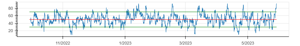

Signal

signal_buy = RSI > 70
signal_sell = RSI < 30
signal = signal_buy.astype(int) - signal_sell.astype(int)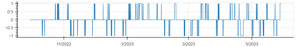

Positions

position = signal.where(signal != 0).ffill() > 0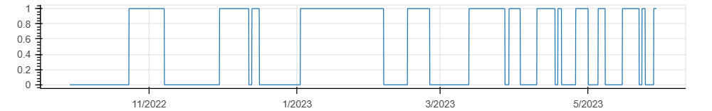

Rendement net cumulé

Code

# coding: utf-8

import numpy as np
import pandas as pd
import talib as ta

df = pd.read_csv('./btceur-2h.csv')

# strategy
RSI = ta.RSI(df.close, timeperiod = 14)
signal_buy = RSI > 70
signal_sell = RSI < 30

# position
signal = signal_buy.astype(int) - signal_sell.astype(int)
position = signal.where(signal != 0).ffill() > 0

# returns
returns_hodl = np.log(df.close / df.close.shift())
returns_strat = returns_hodl * (position.shift() == 1)
returns_fee = np.log(1 - 0.0025) * (position != position.shift())
returns_netto = returns_strat + returns_fee
print('Returns: ', np.exp(returns_netto.sum()))

# graphs
from bokeh.plotting import figure,show
from bokeh.layouts import column,row

df['date'] = pd.to_datetime(df.time, unit='s')

fig0 = figure(height=325, width=800, x_axis_type='datetime')
fig0.line(df.date, df.close)

fig1 = figure(height=125, width=800, x_axis_type='datetime')
fig1.line(df.date, RSI)
fig1.line(df.date, 70, color='green')
fig1.line(df.date, 50, color='red')
fig1.line(df.date, 30, color='green')

fig2 = figure(height=125, width=800, x_axis_type='datetime')
fig2.line(df.date, signal)

fig3 = figure(height=125, width=800, x_axis_type='datetime')
fig3.line(df.date, position)

fig4 = figure(height=325, width=800, x_axis_type='datetime')
position_in = (position == 1) & (position.shift() == 0)
position_out = (position == 0) & (position.shift() == 1)
fig4.line(df.date, df.close, color='lightgray')
fig4.line(df.date, df.close.where(position == 1, np.nan), color='green')
fig4.triangle(df.date, df.close.where(position_in), color='green', size=7)
fig4.inverted_triangle(df.date, df.close.where(position_out), color='red', size=7)

fig5 = figure(height=125, width=800, x_axis_type='datetime')
fig5.line(df.date, returns_hodl)

fig6 = figure(height=125, width=800, x_axis_type='datetime')
fig6.line(df.date, returns_hodl, color='lightgray')
fig6.line(df.date, returns_strat)
fig6.line(df.date, returns_fee, color='red')

fig7 = figure(height=325, width=800, x_axis_type='datetime')
fig7.line(df.date, np.exp(returns_hodl.cumsum()), color='lightgray')
fig7.line(df.date, np.exp(returns_strat.cumsum()))
fig7.line(df.date, np.exp(returns_netto.cumsum()), color='red')

layout = column(fig0, fig1, fig2, fig3, fig4, fig5, fig6, fig7)
show(layout)

Backtesting - Advanced trend following RSI

Indicateur

RSI = ta.RSI(df.close, timeperiod = 14)

Signal long

signal_long_buy = RSI > 80
signal_long_sell = RSI < 50
signal_long = signal_long_buy.astype(int) - signal_long_sell.astype(int)

position_long = signal_long.where(signal_long != 0).ffill() > 0

Signal short

signal_short_sell = RSI < 20
signal_short_buy = RSI > 50
signal_short = signal_short_sell.astype(int) - signal_short_buy.astype(int)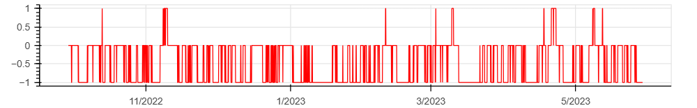

position_short = signal_short.where(signal_short != 0).ffill() > 0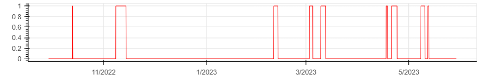

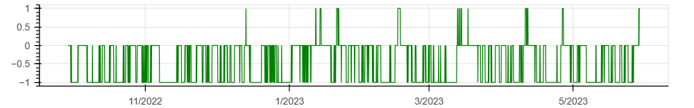
Position

position = position_long.astype(int) - position_short.astype(int)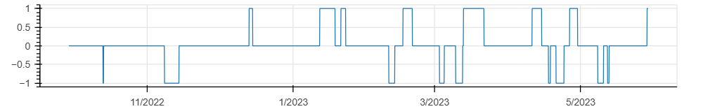

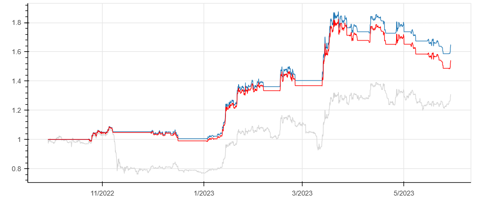
Rendement net cumulé

Code

# coding: utf-8

import numpy as np
import pandas as pd
import talib as ta

df = pd.read_csv('./btceur-2h.csv')

# strategy
RSI = ta.RSI(df.close, timeperiod = 14)
signal_long_buy = RSI > 80
signal_long_sell = RSI < 50
signal_short_sell = RSI < 20
signal_short_buy = RSI > 50

# position
signal_long = signal_long_buy.astype(int) - signal_long_sell.astype(int)
signal_short = signal_short_sell.astype(int) - signal_short_buy.astype(int) 
position_long = signal_long.where(signal_long != 0).ffill() > 0
position_short = signal_short.where(signal_short != 0).ffill() > 0
position = position_long.astype(int) - position_short.astype(int)

# returns
returns_hodl = np.log(df.close / df.close.shift())
returns_strat = returns_hodl * position.shift()
returns_fee = np.log(1 - 0.0025) * (position != position.shift())
returns_netto = returns_strat + returns_fee
print('Returns: ', np.exp(returns_netto.sum()))

# graphic
from bokeh.plotting import figure,show
from bokeh.layouts import column,row

df['date'] = pd.to_datetime(df.time, unit='s')

fig1 = figure(height=325, width=800, x_axis_type='datetime')
fig1.line(df.date, df.close)

fig2 = figure(height=125, width=800, x_axis_type='datetime')
fig2.line(df.date, RSI)
fig2.line(df.date, 70, color='green')
fig2.line(df.date, 50, color='red')
fig2.line(df.date, 30, color='green')

fig3 = figure(height=125, width=800, x_axis_type='datetime')
fig3.line(df.date, signal_long, color='green')

fig4 = figure(height=125, width=800, x_axis_type='datetime')
fig4.line(df.date, position_long, color='green')

fig5 = figure(height=125, width=800, x_axis_type='datetime')
fig5.line(df.date, signal_short, color='red')

fig6 = figure(height=125, width=800, x_axis_type='datetime')
fig6.line(df.date, position_short, color='red')

fig7 = figure(height=125, width=800, x_axis_type='datetime')
fig7.line(df.date, position)

fig8 = figure(height=325, width=800, x_axis_type='datetime')
position_long_in = df.close.where((position == 1) & (position.shift() != 1))
position_long_out = df.close.where((position != 1) & (position.shift() == 1))
position_short_in = df.close.where((position == -1) & (position.shift() != -1))
position_short_out = df.close.where((position != -1) & (position.shift() == -1))
fig8.line(df.date, df.close, color='gray')
fig8.triangle(df.date, position_long_in, color='cyan', size=7)
fig8.inverted_triangle(df.date, position_long_out, color='blue', size=7)
fig8.inverted_triangle(df.date, position_short_in, color='orange', size=7)
fig8.triangle(df.date, position_short_out, color='red', size=7)
fig8.line(df.date, np.where(position == 1, df.close, np.nan), color='green')
fig8.line(df.date, np.where(position == -1, df.close, np.nan), color='red')

fig9 = figure(height=150, width=800, x_axis_type='datetime')
fig9.line(df.date, returns_hodl, color='lightgray')
fig9.line(df.date, returns_strat)
fig9.line(df.date, returns_fee, color='red')

figa = figure(height=325, width=800, x_axis_type='datetime')
figa.line(df.date, np.exp(returns_hodl.cumsum()), color='lightgray')
figa.line(df.date, np.exp(returns_strat.cumsum()))
figa.line(df.date, np.exp(returns_netto.cumsum()), color='red')

layout = column(fig1, fig2, fig3, fig4, fig5, fig6, fig7, fig8, fig9, figa)
show(layout)